3.2.3. Inversion Input File

Important

Both the forward and inverse problems are solved using the mtz3d.exe executable program. In both cases, the lines of the input file are the same. However in the case of forward modeling, some lines in the input file are not used by the code and can be given any value. The input file for forward modeling and inversion must be given the name mt3dinv.inp!!!

The lines of input file for mtz3d.exe are as follows:

Line #	Description	Description
1	Tensor mesh	path to tensor mesh file
2	Background conductivity	set background conductivity for
3	Survey file	path to observations/locations file
4	Initial/FWD model	initial model
5	Reference model	reference model
6	Background susceptibility	background susceptibility model
7	Active model	sets active cells in inversion
8	Bounds	upper and lower bounds for cells
9	Sensitivity weights	additional cell weights
10	Trade-off parameter settings	cooling schedule for beta parameter
11	alpha_s alpha_x alpha_y alpha_z	weighting constants for smallness and smoothness constraints
12	Reference model	stopping criteria for inversion
13	Hard constraints	set the number of Gauss-Newton iteration for each beta value
14	Model type	set the tolerance and number of iterations for Gauss-Newton solve
15	Chi factor	reference model
16	Methpar	use SMOOTH_MOD or SMOOTH_MOD_DIFF
17	tol_nl mindm iter_per_beta	upper and lower bounds for recovered model
18	into max_linit	set solver parameters for iterative inversion
19	fortol initol	set solver parameters for iterative inversion
20	max_it_bicg droptol droptol_WTW	set BICG tolerances

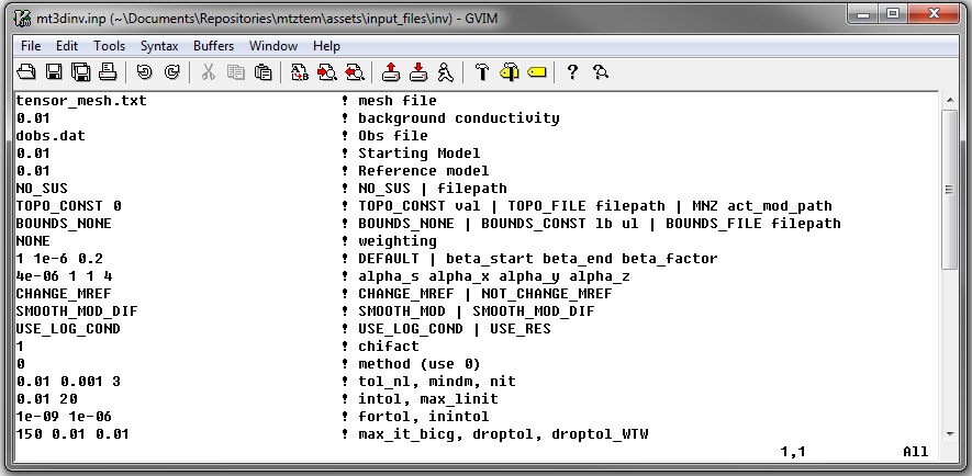
Fig. 3.2 Example input file for the inversion (Download ). Example input file for the forward modeling (Download ).

3.2.3.1. Line Descriptions

• Tensor Mesh: file path to a tensor mesh file

• Background Conductivity:

  • The user may supply the file path to a 1D background conductivity model .

  • If a homogeneous background conductivity is being used, the user enters the value in S/m.

• Survey File: file path to the observations/locations file.

• Initial/FWD Model: On this line we specify either the starting model for the inversion or the conductivity model for the forward modeling. On this line, there are 3 possible options:

  • If the program is being used to forward model data, the flag ‘FWDMODEL’ is entered followed by the path to the conductivity model.

  • If the program is being used to invert data, only the path to a conductivity model is required; e.g. inversion is assumed unless otherwise specified.

  • If a homogeneous conductivity value is being used for all active cells, the user can enter the value in S/m.

Important

If data are only being forward modeled, only the background susceptibility model, topography, fortol and bicg solver parameters are required. However, the remaining fields must not be empty and must have correct syntax for the code to run.

• Reference Model:

  • The user may supply the file path to a reference conductivity model.

  • If a homogeneous conductivity value is being used for all active cells, the user can enter the value in S/m.

• Background Susceptibility Model:

  • The user may supply the file path to a background susceptibility model.

  • If a homogeneous susceptibility value is being used for all active cells, the user can enter the value in SI.

  • If the Earth is non-magnetic, the user may use the flag “NO_SUS”.

• Active Model: Here, the user can choose to specify the cells which are active in forward modeling and inversion. To set the active cells, there are 3 options:

  • use the flag TOPO_CONST followed by the value in meters if the active cells lie below a flat topography

  • use the flag TOPO_FILE followed by the file path to a topography file

  • use the flag MNZ followed by the file path to an active cells model file

Important

If TOPO_CONST or TOPO_FILE options are used, then all cell lying above surface topography are given physical property values of \(\sigma = 10^{-8}\) S/m and \(\chi=0\) SI during forward modeling or inversion. If MNZ is used, the inactive cells (0 in the active model) are set to the values of the reference model.

• Bounds:

  • use the flag “BOUNDS_NONE” for no upper and lower bounds on recovered conductivities

  • use the flag “BOUNDS_CONST” followed by a value for the lower and upper bounds, respectively, to apply the same bounds to all cells (example: BOUNDS_CONST 1E-10 0.1)

  • use the flag “BOUNDS_FILE” followed by the file path to a bounds file

• Sensitivity Weights: Here, the user specifies whether sensitivity weighting is applied. To set the sensitivity weighting:

  • use the flag NONE if no sensitivity weighting is being applied

  • or provide the filepath to a weights file

• Trade-Off Parameter Settings: Here, the user specifies the protocols for the trade-off parameter (beta). beta_start is the initial value of beta, beta_end is the minimum allowable beta the program can use before quitting and beta_factor defines the factor by which beta is decreased at each iteration; example “1E4 10 0.2”. The user may also enter “DEFAULT” if they wish to have beta calculated automatically. See theory section for cooling schedule.

• alpha_s alpha_x alpha_y alpha_z: Alpha parameters . Here, the user specifies the relative weighting between the smallness and smoothness component penalties on the recovered models. As a default setting, alpha_x=alpha_y=alpha_z=1 and alpha_s=1/h \(\!^2\) is suggested, where h is the average dimension of cells in the core region.

• Reference Model Update: Here, the user specifies whether the reference model is updated at each inversion step result:

  • use the flag CHANGE_MREF if the reference model is updated at each iteration

  • use the flag NOT_CHANGE_MREF for the reference model to remain the same throughout the entire inversion

• Hard Constraints: Here, the user specifies whether how the reference model is used to constrain the inversion; go to fundamentals of inversion to see how this is implemented. For the MTZTEM package:

  • use the flag SMOOTH_MOD to ignore the reference model (essential set \(m_{ref}=0\) )

  • use the flag SMOOTH_MOD_DIF to include \(m_{ref}\) in the smallness and smoothness penalty terms

• Model Type: Here, the user specifies whether the model representing the Earth’s conductivity is a log-conductivity or electrical resistivity model. Although the output model is a conductivity model, this choice will have an impact on how the sensitivity is computed:

  • use the flag USE_LOG_COND to define the model as a log-conductivity model

  • use the flag USE_RES to define as an electrical resistivity model

Note

It is suggested that USE_LOG_COND be used unless there is reason to do otherwise.

• Chi Factor: The chi factor defines the target data misfit for the inversion. Once the target misfit is reached, the recovered model fits the field observations sufficiently without fitting the noise and the inversion ceases. A chi factor of 1 means the target misfit is equal to the total number of data observations. For more, see fundamentals of inversion .

• Methpar: This line is used to specify parallelization options. Currently, only one option is available and this line should be set to a flag of 0 .

• tol_nl mindm iter_per_beta: Here, the user specifies parameters related to the number of Newton iterations at each trade-off parameter (\(\beta\) ) value. tol_nl is a tolerance on Newton iterations. The model is considered optimal when the gradient components of the current iteration are sufficiently smaller than those of the initial iteration multiplied by the tolerance. mindm is the minimum model perturbation. The Newton iterations stop when if the largest value in the current model is smaller than mindm . iter_per_beta maximum number of Newton iterations for a fixed trade-off parameter. To set these parameters:

  • use the flag DEFAULT, in which case tol_nl = 0.01, mindm = 0.001 and iter_per_beta = 5.

  • or set tol_nl, mindm and iter_per_beta in order separated by spaces

• intol max_linit: Here, the user specifies solver parameters. intol specifies the tolerance for the linear solver (ipcg). This parameters find the optimal model perturbation size (typically between 0.001 and 0.1). max_linit sets the maximum number of iterations for the linear solver.

  • use the flag DEFAULT, in which case intol = 0.01 and max_linit = 10

  • or set intol, and max_linit in order separated by spaces

• fortol initol: the parameter fortol sets the stop tolerance for forward and adjoint calculations when evaluating the objective function and gradients. This should be very small (\(\sim 10^{-9}\) ). initol sets the stop tolerance for the forward and adjoint calculations inside the linear solver (ipcg). This tolerance can be larger than “fortol” to save time (typical 0.001 and lower).

  • use the DEFAULT flag, in which case fortol = \(10^{-9}\) and initol = \(10^{-8}\)

  • or set fortol, and initol in order separated by spaces

• max_it_bicg droptol droptol_WTW: Here, max_it_bicg set the maximum number of iterations in BiCGSTAB when performing the forward and adjoint calculations. droptol sets the drop tolerance for the ILU preconditioner for the A matrix. And droptol_WTW sets the drop tolerance for the ILU preconditioner for the WTW matrix. This is used when the algorithm is looking for optimal model step size, and in the IPCG solver.

  • use the DEFAULT flag, in which case max_it_bicg = 15, droptol = 0.01 and droptol_WTW = 0.01

  • or set max_it_bicg, droptol and droptol_WTW in order separated by spaces